How to make a consolidated table in Excel 2003, 2007, 2010 with Formulas: Step-by-step instructions

People who have attended work through the Internet and not only, probably often stumbled upon vacancies, where the main requirement for the applicant was a confident knowledge of the Microsoft Office program package, and in particular the program Microsoft Excel..

The thing is that at certain positions, people have to work with a large number of data, and Microsoft Excel program allows you to organize them in tables and graphically present information. That is why to know the foundations of this program will not hurt anyone.

Specifically for those people who just started to know Microsoft Excel., we wrote this article. It will be discussed about such an important program tool as " Consolidated tables" It is with the help of these tables that the data are sorted and accounting them.

Step-by-step instructions for creating consolidated tables with formulas in Microsoft Excel

What are consolidated tables in Excel and what are they needed for?

Summary calls that tables that contain parts of the data and show them so that the relationship between these data is clearly visible. In other words, these tables allow you to keep accounting for something in a convenient form. It is best to explain on the example:

• Imagine that you are the owner of a small clothing store, in which several sellers work. You need to determine the activity of each of them.
• To do this, you will need to allocate several indicators: the name of the seller sold by them the goods, the date of sale and the amount of revenue. You open Excel, share the work field into four columns and in each of these columns recording daily sales rates. It looks like this as follows:

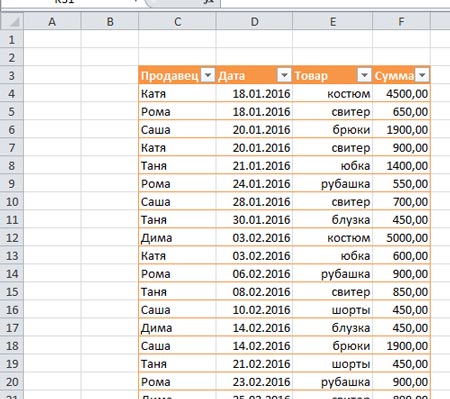
Figure 1. What is consolidated tables in Excel and what are they needed for?

• Agree, such a graphical method of presenting data is very simple and easy to read? However, the graphic component of the consolidated table is not completed.
• If you look carefully, then in the table header next to each header you can notice the arrow. If you click on it, you can sort the table data by selected parameters.
• For example, you can choose only the seller Katya and look at the goods sold by it, sales and amounts. Similarly, you can sort sales by date. Choosing a date, you will see sellers who sold goods on that day and the total amount of day revenue.

What is Formulas in Excel and what are they needed for?

• The word "formula" is all familiar to us since school years. IN Excel Formulas prescribe a specific procedure with numbers or values \u200b\u200bthat are in cells. The whole essence of the spreadsheet is in the formulas. After all, without them, they lose all meaning of their existence.

For formulas in Microsoft Excel, standard mathematical operators are used:

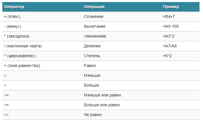
Figure 1. What is the formula in Excel and what are they needed for?

• During multiplication, you must always use the sign " *" His omission, as in the written embodiment, is unacceptable. In other words, if you write down (4+7)8, then this entry program will not be able to recognize, since after the round bracket is not a sign of multiplication " *».
• The Excel program is used by many instead of a calculator. For example, if you enter the formula row 2+3The result will display the result in the selected cell. 5.

Figure 2. What is the formula in Excel and what are they needed for?

• However, when creating a summary tables for formulas, links to cells with values \u200b\u200bare used. When a value is changed in the cell, the formula will automatically recalculate the result.

Figure 3. What is the formula in Excel and what are they needed for?

Creating a database for making it into a consolidated table Excel 2003, 2007, 2010

We have already figured out that consolidated tables have solid advantages. However, in order to proceed with creating them, it is necessary to have an already accumulated database, which will be entered in the table.

As Excel A rather complicated program with a large set of tools and functions, we will not deepen into its study with your head, but only show the general principle of creating a database. So, proceed:

Step 1.

• Run the program. On the main page, you will see a standard field with cells where you need to drive our database.
• First you need to create four basic columns with headlines.
• For this, double click on one of the top cells and enter the name of the first title in it. Seller" and press ENTER.
• Next, do the same with three adjacent cells in the same line, entering the title names in them.

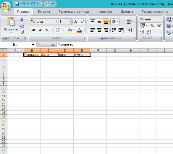
Figure 1. Creating a database for making it to a consolidated table Excel 2003, 2007, 2010

Step 2..

• After you have entered the title names, you need to increase the font size and make fat so that they stand out against the background of other data.
• To do this, clamp the left mouse button on the first cell and enter the mouse to the right, highlighting the neighboring three.
• After allocating all cells on the working panel with the text, set the font size for them. 12, Highlight it fatty and align on the left edge.
• The text will certainly be placed in the cells, so tighten the left mouse button on the border of the cell and move the mouse to the right, thereby increasing it.
• You can do the same with the height of cells.

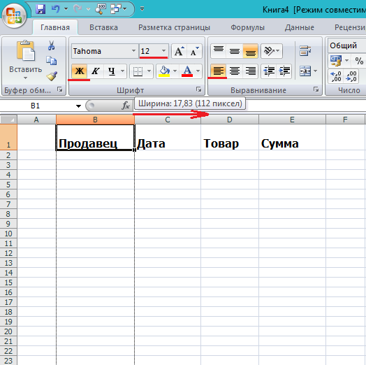
Figure 2. Creating a database for making it into a consolidated table Excel 2003, 2007, 2010

Step 3..

• Next, under each title, enter the corresponding parameter in exactly the same way as you entered the headlines.
• In order not to suffer with the editing of each cell, after entering the parameters, select them all with the mouse and apply the same properties to them directly.

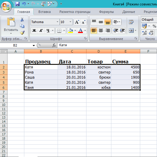
Figure 3. Creating a database for making it into a consolidated table Excel 2003, 2007, 2010

How to make a consolidated table in Excel 2003, 2007, 2010 with formulas?

Now that you have a database, you can go directly to creating a pivot table. To do this, do the following steps:

Step 1.

• First of all, it is necessary to highlight one of the cells you have the starting table. Next in the upper left corner, go to the " Insert"And click on the button" Summary Table».

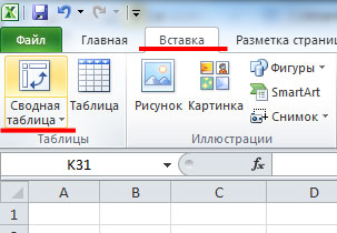
Figure 1. How to make a consolidated table in Excel 2003, 2007, 2010 with formulas?

Step 2..

• You will open the window in which you need to select a range or enter the table name.
• Also in the window there is the ability to select a place to report. Create it on a new sheet.
• Mark points items that are listed on the screenshot below and click the " OK».

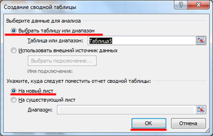
Figure 2. How to make a consolidated table in Excel 2003, 2007, 2010 with formulas?

Step 3..

• You will open a new sheet to which another empty table will be placed. On the right side of the window will appear column with fields and areas.
• Under the fields, the headers of the columns that are inscribed in your initial table with the data are implied. You can drag them with the mouse to the existing areas, which will allow you to form a consolidated table.
• The headlines involved will be dawn. In one area you can make several headers and change their locations in order to obtain the most acceptable type of data sorting.

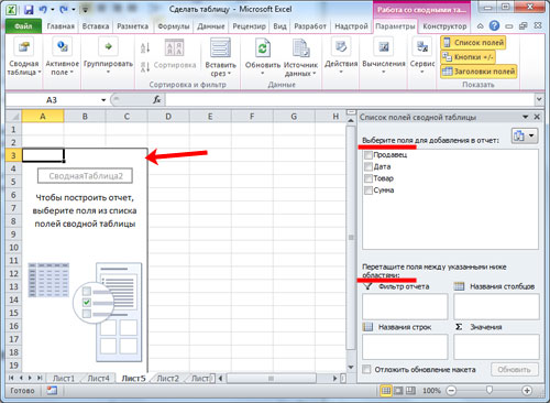
Figure 3. How to make a consolidated table in Excel 2003, 2007, 2010 with formulas?

Step 4..

• Next, it is necessary to decide what we want to analyze. For example, we want to understand what specifically the seller, sold what product for a certain period of time and how much. Data filtering in the table will be carried out on sellers.
• In the spray column, select the title " Seller", Hold the left mouse button on it and drag into the area" Filter report».
• As you can see, the appearance of the table has changed, the title became marked.

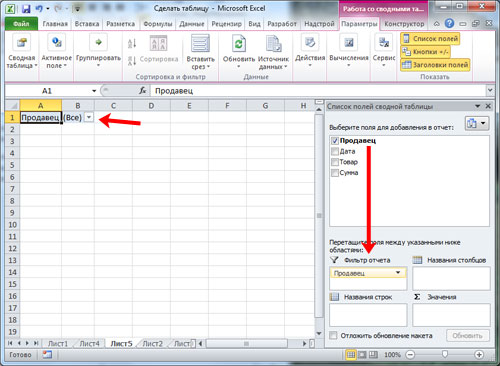
Figure 4. How to make a consolidated table in Excel 2003, 2007, 2010 with formulas?

Step 5..

• Next, on the same scheme in the spray column, you must clamp the left mouse button on the title " Products"And drag it to the area" Row names».

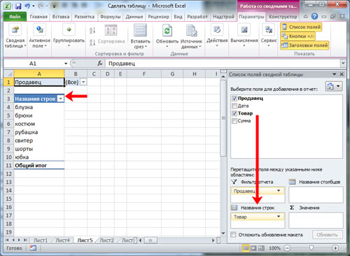
Figure 5. How to make a consolidated table in Excel 2003, 2007, 2010 with formulas?

Step 6..

• Next to the column " Names of columns»Let's try to drag the title" date».
• To make a list of sales to be displayed not daily but, for example, monthly, you must click on any cell with the date of the right mouse button and select from the list item " Group».

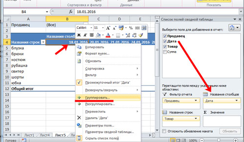
Figure 6. How to make a consolidated table in Excel 2003, 2007, 2010 with formulas?

• In the window that opens, you will need to select a grouping period (which is the number for what), and select a step from the list. After which you should click " OK».

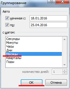
Figure 7. How to make a consolidated table in Excel 2003, 2007, 2010 with formulas?

• Next, your table is converted so that way.

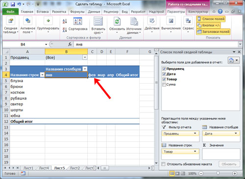
Figure 8. How to make a consolidated table in Excel 2003, 2007, 2010 with formulas?

Step 7..

• Next item Pull the title " Sum"In the column" Value».
• As you can see, it was simply displayed, despite the fact that the display format was applied to this column in the table in the starter version of the table. Numerical».

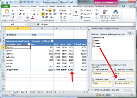
Figure 9. How to make a consolidated table in Excel 2003, 2007, 2010 with formulas?

• To correct this problem, select the necessary cells in the pivot table, right-click from the list click on the point " Numeric format».

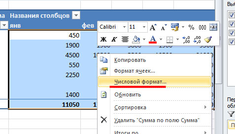
Figure 10. How to make a consolidated table in Excel 2003, 2007, 2010 with formulas?

• In the window that opens in the section " Conditional formats"Select" Numerical"And you can optionally note the checkbox" Separator of discharge groups».
• Next click " OK" As you can see, simple numbers have changed and are not simply displayed. 650, but 650,00.

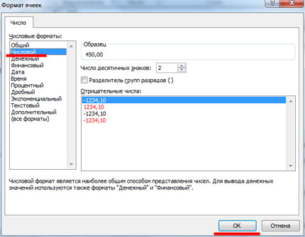
Figure 11. How to make a consolidated table in Excel 2003, 2007, 2010 with formulas?

Step 8..

• In theory, the consolidated table is ready and you can start working with it. For example, when choosing a seller, you can choose one, two, three or immediately all, putting a marker opposite item " Mark multiple elements».

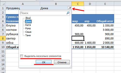
Figure 12. How to make a consolidated table in Excel 2003, 2007, 2010 with formulas?

• In exactly the same way, you can filter lines and columns. For example, the names of goods and the date.
• Noting the field checkboxes Pants"And" Costume", It is easy to figure out how many sales of their sales are revenue in general, or specific sellers.

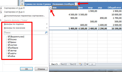
Figure 13. How to make a consolidated table in Excel 2003, 2007, 2010 with formulas?

• Also in the column " Values»You can set certain parameters header. At the moment there is a parameter " Sum».
• That is, if you look at the table, you can see that the seller Roma in February was sold shirts for a total amount 1 800,00 rubles.
• In order to find out their quantity, you need to click on the mouse on the point " Sum"And choose from the line menu" Parameters of fields of values».

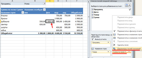
Figure 14. How to make a consolidated table in Excel 2003, 2007, 2010 with formulas?

• Next opens the window where you need to select " number"And click the" OK" After that, your table will change and, looking at it, you will understand that for February, the novel sold his shirts in the number of two pieces.

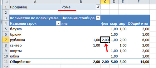
Figure 15. How to make a consolidated table in Excel 2003, 2007, 2010 with formulas?

As already above, the program was stipulated. Excel It has an extensive range of tools and opportunities, so it is possible to talk about working with tables to infinity.

In order to better understand it, we advise you to sit on your own and experiment with changes in values. If that you will be incomprehensible, refer to the built-in help Microsoft Excel.. It is exhaustive in it.

Video: Creating a pivot table in Excel