
How to use the PRD function in Excel: understandable instructions for teapots, video, comparison of two tables, drop-down list, examples. Formula Functions of the PRD in Excel: examples, several conditions, decoding
Article Article: "EPS Function in Excel for Doodles".
Navigation
PRD Function in Excel makes it possible to rearrange the data of one table to another in cells. This is a very popular and convenient way, and we will talk about it in today's review.
PRD Function in Excel: instructions for teapots
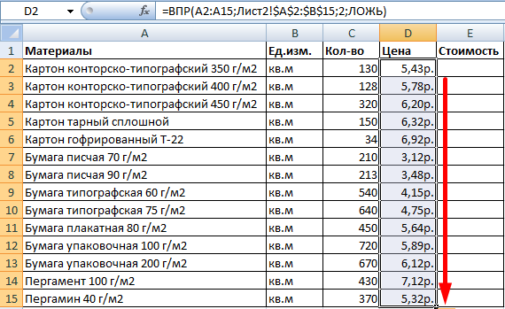
Suppose we have the following task. Our factory brought the materials you need, which are presented in the following table:
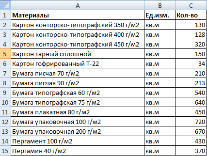
Table in "Excel"
In another table, we have the same list indicating the value of these materials:
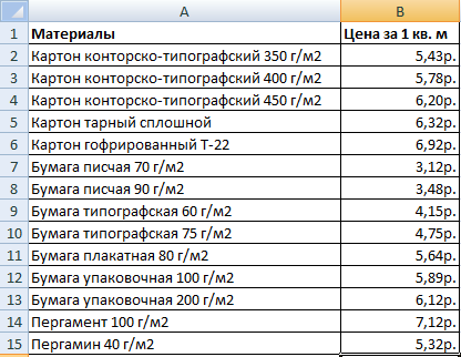
Price list in "Excel"
That is, in the first table we have the number of materials, and in the second - the cost of the piece (rub / sq.m). Our task, calculate the total cost of all materials that were brought to the factory. To do this, we need to postpone the indicators from the second table in the first and with the help of the multiplication to find the answer.
We will proceed to the case:
- In the first table we lack two columns - " Price"(That is, the cost per 1 sq. M) and" Cost"(I.e., the total cost of the brought material). Add these columns. Now highlight in the column " Price»Upper first cell, run" Master of Functions"(Press simultaneously" F3."And" Shift."), In the tab" Formulas" Press " Links and arrays"And in the dropping list, select" Pr».

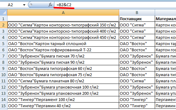
Run the "Function Wizard", in the "Formula" tab, click on "Links and arrays" and in the dropping list, select "VDP"
- Further in the new window that opens opposite the item " Secondary value»We observe the following indicators: A1: A15. That is, the program records the name of the names of materials in the corresponding post " Materials" The same program should show both in the second table.

We observe the following indicators: A1: A15
- Now we'll figure it out with the second point - " Table"(The second table with the cost of materials). Click on this item, then highlight the names of materials in the second table along with prices. As a result, the result should be as follows.

Click on "Table"
- Next, select the results in the " Table"And click on" F4.", After which they will appear in them." $"- Thus, the program will refer to the indicators in" Table».
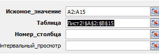
Highlight the results in the "Table" point and click on "F4"
- Next, go to the third item - " Column number" Specify here " 2" In the last fourth paragraph " Interval view»Specify" FALSE" After all these manipulations click on " OK».
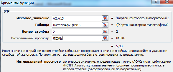
In the last fourth paragraph "Interval View", specify "Lie"
- Finishing touch. Mouse cursor Press the bottom right corner of the table and pull down the time until you see a full list of material names along with prices.
Mouse cursor Press the bottom right corner of the table and pull down
All, we have tied both our tables. Calculate the total cost of materials will be easier than simple. Now we need to take into account that if the price list changes, the results we receive will change. Therefore, we need to avoid this with the following actions:
- Highlight all the indicators in the column " Price", Click on it right mouse button and then - on" Copy».
- Right-click on already dedicated prices again and then on " Special insert».
- In the window that opens, check the daw, as shown in the screenshot, and click on " OK»
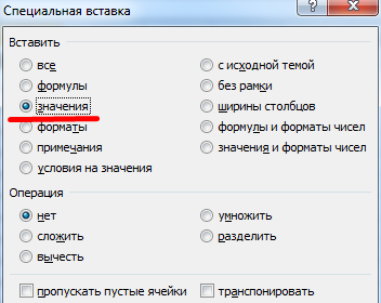
Check the "Values"
Compare two tables using the PRD function in Excel
Suppose the price list has changed, and we need to compare two tables - new and old prices:
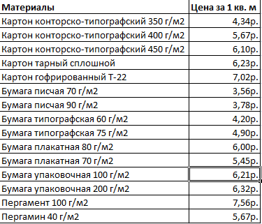
Price list
To do this, we use the corresponding function in " Excel»:
- In the old table, add a column " New price»

Add a column "New price"
- Next, we repeat the actions that we made above - allocate the first upper cell, choose " Pr", in point " Table»We get results and click on" F4.».

in the table "Table" we obtain the following results
- That is, in the screenshot above, we observe that from the table with new prices, we transferred the cost of each material into the old table and obtained the following results.
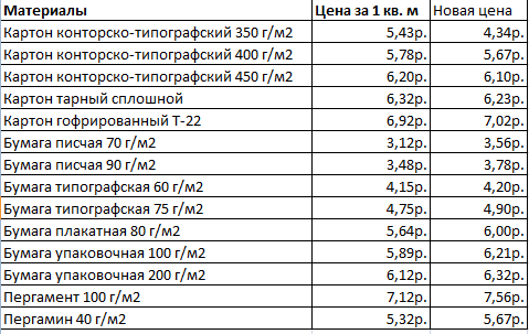
Table
We work with multiple conditions using the PRD function in Excel
Above we worked with one condition - the name of the materials. But in reality, circumstances may be different. We can get a table with two or more conditions, for example, both with the name of the materials and the name of their suppliers:
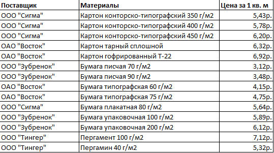
Table with the names of suppliers and materials
Now our task is complicated. Suppose we need to find at what price this or that material is separately taken by the supplier. An even more difficult to be the situation when the supplier sells several materials, while the suppliers themselves may also be somewhat.
Let's try to solve this task:
- Add the left extreme column to the table and combine two columns - " Materials"And" Suppliers».
Combine two columns - "Materials" and "Suppliers"
- Similarly, combine the desired request criteria
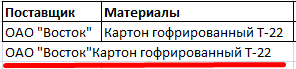
Combine the desired request criteria
- Again in paragraph " Table»Set the appropriate indicators

In the "Table" paragraph, set such indicators
- In the screenshot above, we see the following formula (1 - the search object; 2 - the search place; 3 - the data taken by us).
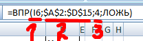
1 - search object; 2 - search place; 3 - these data
We work with a drop-down list
Suppose we have certain data (for example, " Materials") Show in the drop-down list. Our task is to see also worth seeing the cost.
For this, we will take the following steps:
- Press the mouse to the cell " E8."And in the tab" Data»Choose" Data check»

Click on "Data Check"
- Next in the tab " Parameters»Select" List"And click on" OK»
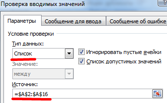
Select "List" and click on "OK"
- Now in the drop-down list we see the item " Price»
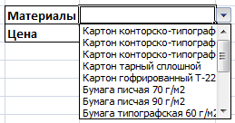
Get the item "Price"
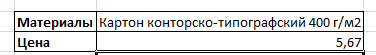
- Next, we need in front of the point " Price»Explanted material cost
- Click on the cell " E9.", in " Wizard functions»Select" Pr" Opposite item " Table»Must be exhibited as follows.

In the "Table" must be as follows
- Press " OK"And get the result
We get results